2.1. The CLMS

The Copernicus Land Monitoring Service (CLMS) is part of the Copernicus programme and it aims to provide geographical information on land use and land cover with its changes, ground motion, vegetation state, water cycle and earth surface energy variables. All in a pan-European and global context. All products are free of charge and can be used for any purpose. Once you have opened the CLMS website you will be greeted by its homepage (Fig. 2.1.1). From the top bar of the homepage you can go to other sections of the website devoted to: seek technical assistance (1), view product updates (2), check news and events (3) (these can be directly checked in the homepage) and take a look at work opportunities (4). You can also register a new account or log in (5): how to do so, will be shown in Fig. 2.1.1.2. Lastly, it is possible to search directly for the information you are interested in by using the search bar (6). It is also possible to reach the main pages of the website using the main menu (7), those pages will be discussed further below. By clicking on the listed product types (8) you will be brought to the Data Viewer page already filtered by the products you have selected. Datasets are grouped into categories, including:

• land cover and land use mapping, consisting of land cover classifications and layers on vegetated land cover characteristics;
• priority area monitoring, including land cover/land use information for specific areas of interest prone to environmental changes;
• bio-geophysical parameters, encompassing layers on the status and evolution of the land surface, complemented by the long-term time series;
• ground motion monitoring, including information on the natural and anthropogenic ground motion;
• satellite data, that is, satellite image mosaics from Copernicus and commercial satellite missions for land surface conditions monitoring;
• reference and validation data, consisting of ground-based observations that can be used as geospatial reference data.

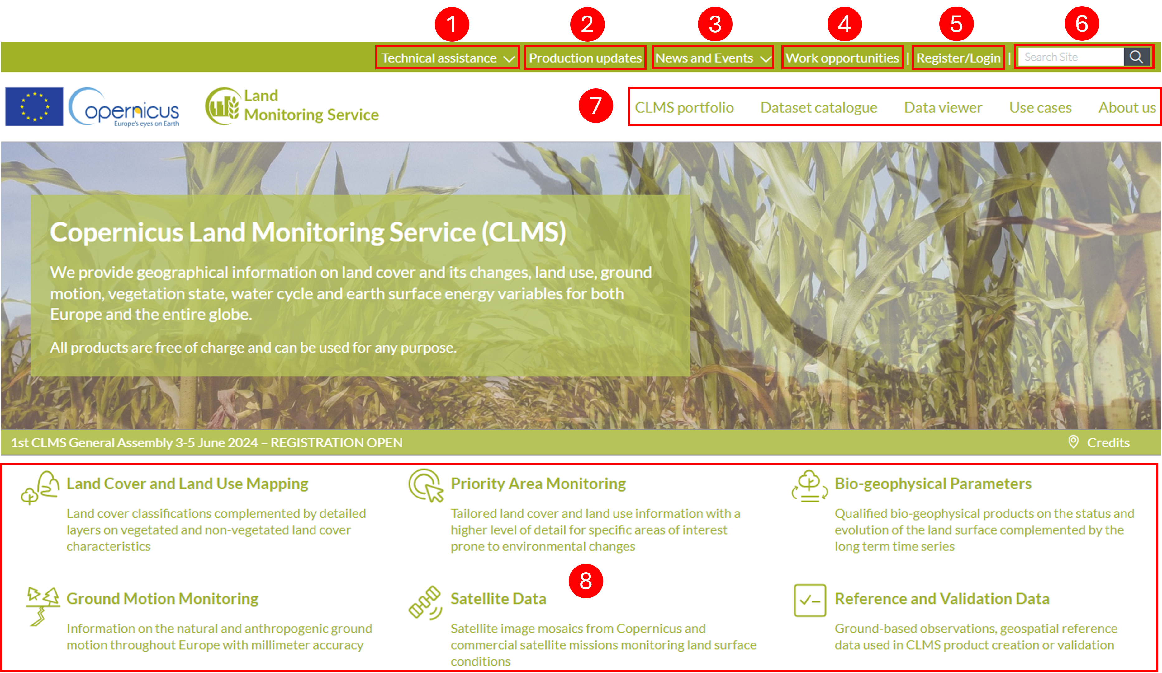
Fig. 2.1.1 – CLMS website - homepage pt.1

Scrolling down the webpage you will see two main buttons (Fig. 2.1.2), one will bring you to the Dataset catalogue page (1) and the other to the Data Viewer page (2). It is also possible to take a look at all news, events and product updates by moving through the respective tabs (3).

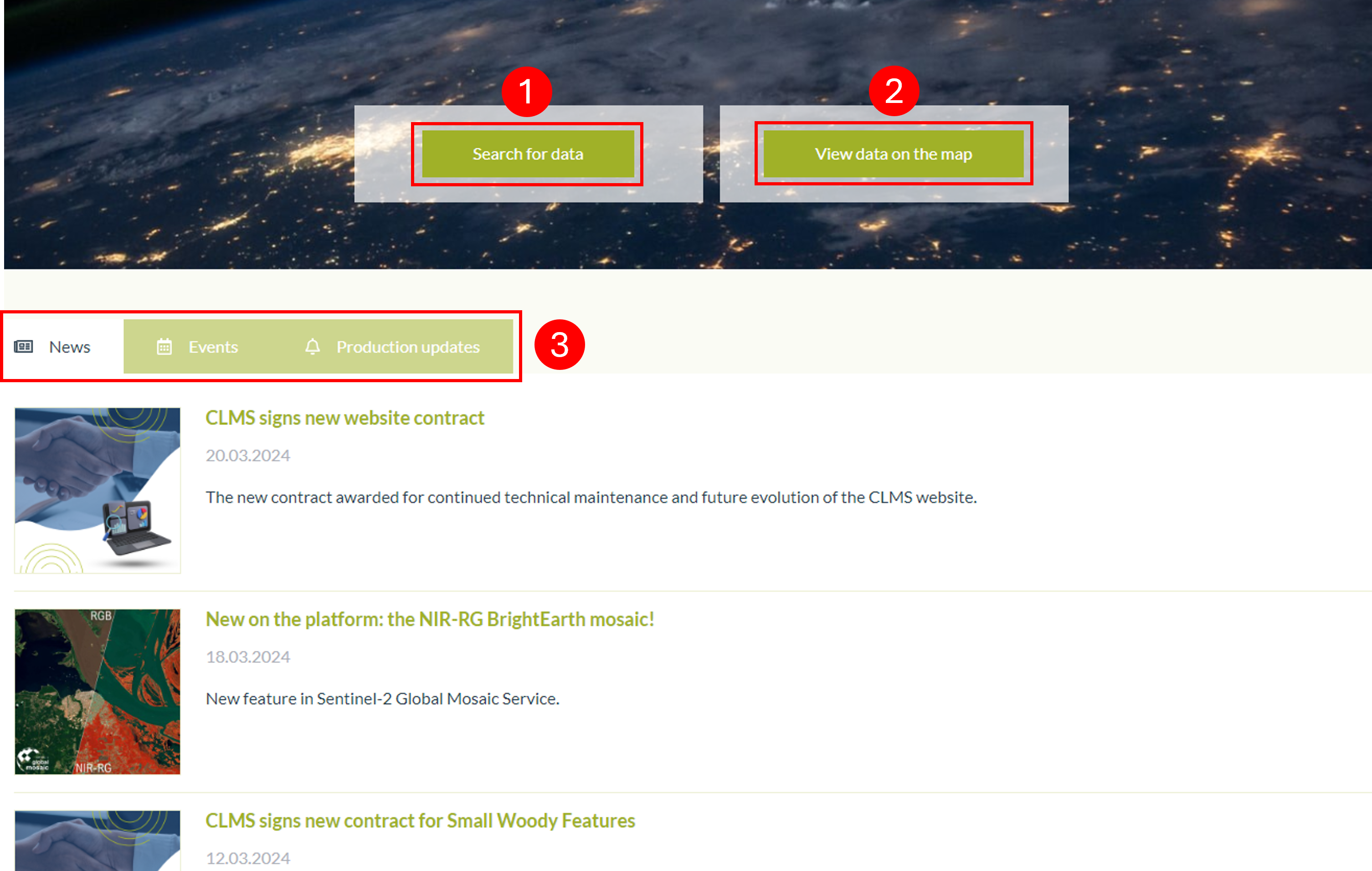
Fig. 2.1.2 – CLMS website - homepage pt.2

Scrolling further down we reach the end of the homepage (Fig. 2.1.3). Here users of the CLMS are presented and it is also possible to open the Use Cases page (1). At the very bottom of the page, there is a section with more technical information (2) grouping: Disclaimer, Data Policy, Personal data protection, Cookies and finally a Sitemap, opening this last page shows the complete structure of the site itself.

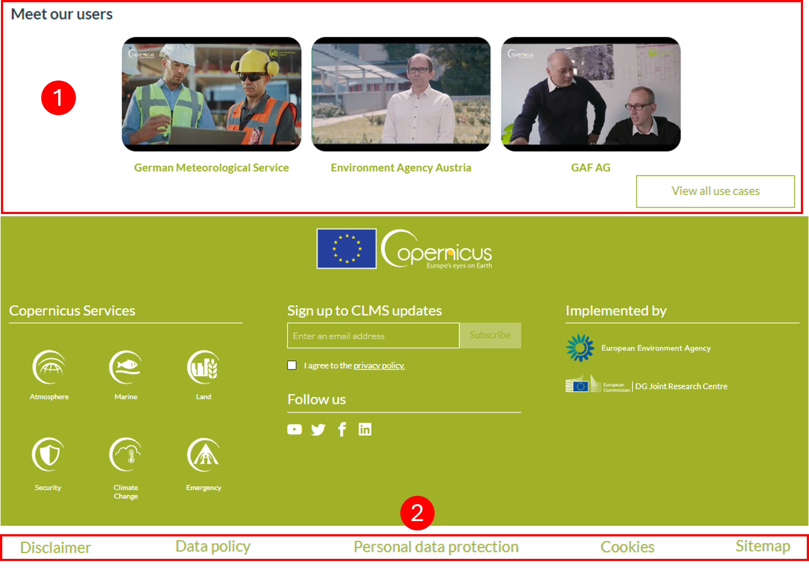
Fig. 2.1.3 – CLMS website - homepage pt.3

From the homepage, we can open the CLMS portfolio page (Fig. 2.1.4) by clicking on CLMS portfolio (1). By default, the Get Overview section will be open (2). In this section, it is possible to open and read a brief overview of all CLMS products containing a description and other information that depends on the product type such as reference year, geographic coverage, update frequency, scale, spatial resolution Minimum Mapping Unit (MMU) and EO data sources.

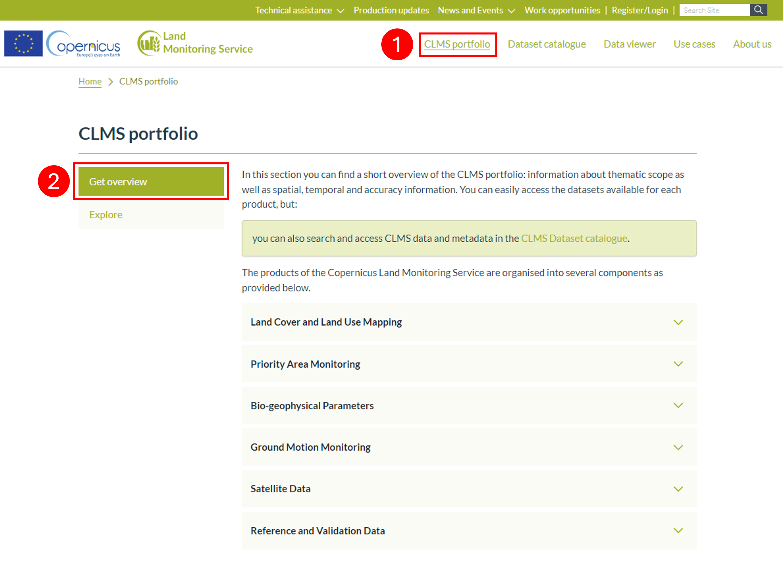
Fig. 2.1.4 – CLMS website - CLMS portfolio pt.1

Opening the Explore tab (Fig. 2.1.5) (1) will allow you to see and subsequently open each product page. By clicking on Filters (2) a lateral bar will open (3) where it is possible to select a subset of all products by ticking boxes (4).

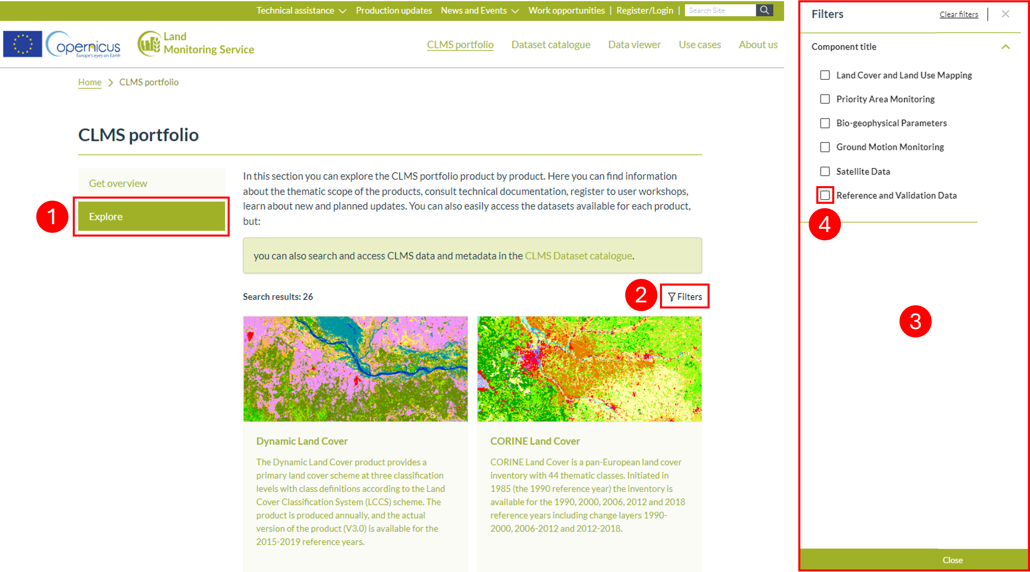
Fig. 2.1.5 – CLMS website - CLMS portfolio pt.2

Clicking on Dataset catalogue (1) (Fig. 2.1.6) we open the homonymous page. This page is similar to the DLMS portfolio one but shows a list of all data. It is possible to find the desired product by using the search bar (2) and/or by clicking on the Filters (3) and selecting the parameters from the lateral menu that will open up (4).

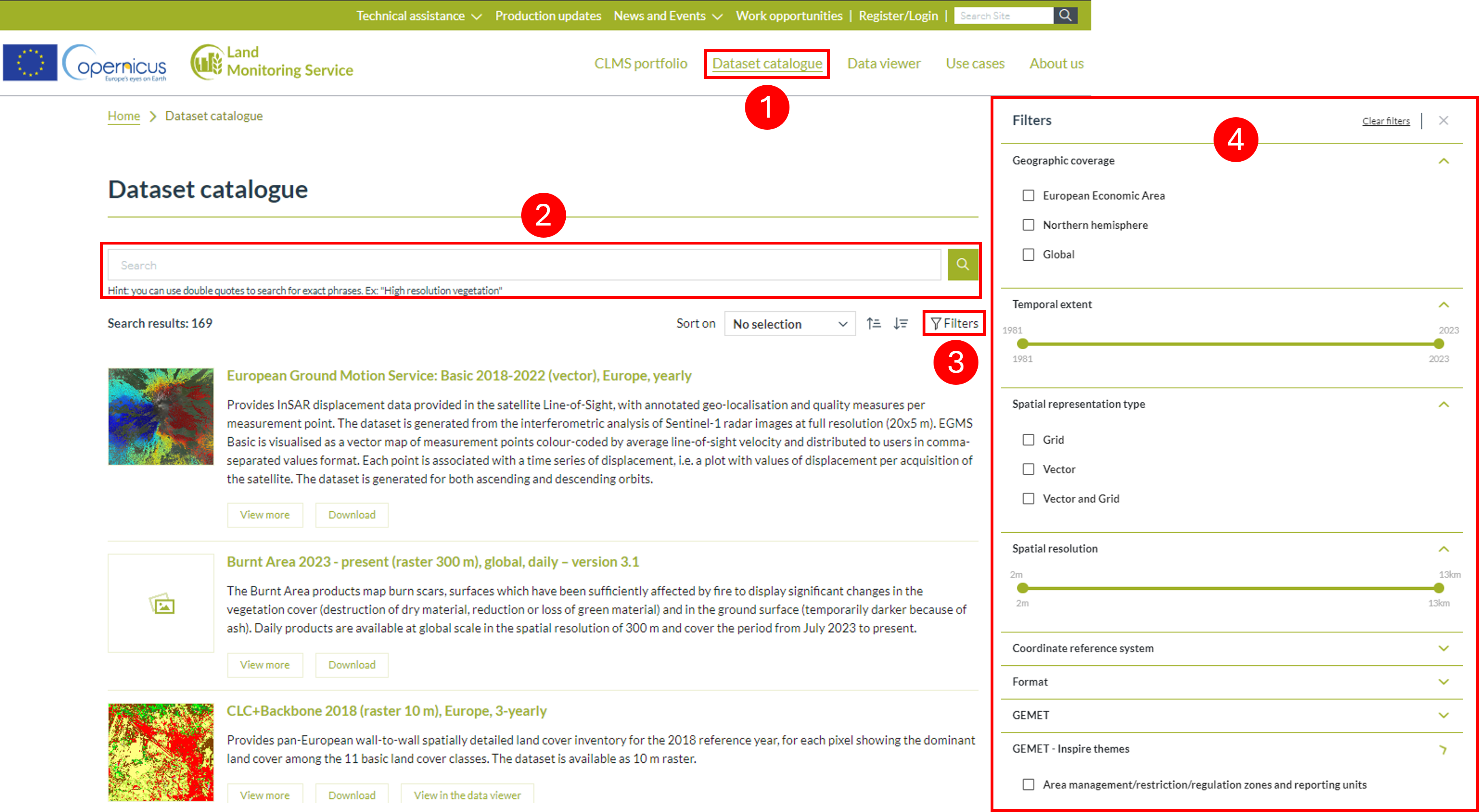
Fig. 2.1.6 – CLMS website - Dataset catalogue

From the Data Viewer page (1) (Fig. 2.1.7) we can visualize data, we will show more about the many offered options in Fig. 2.1.1.1.

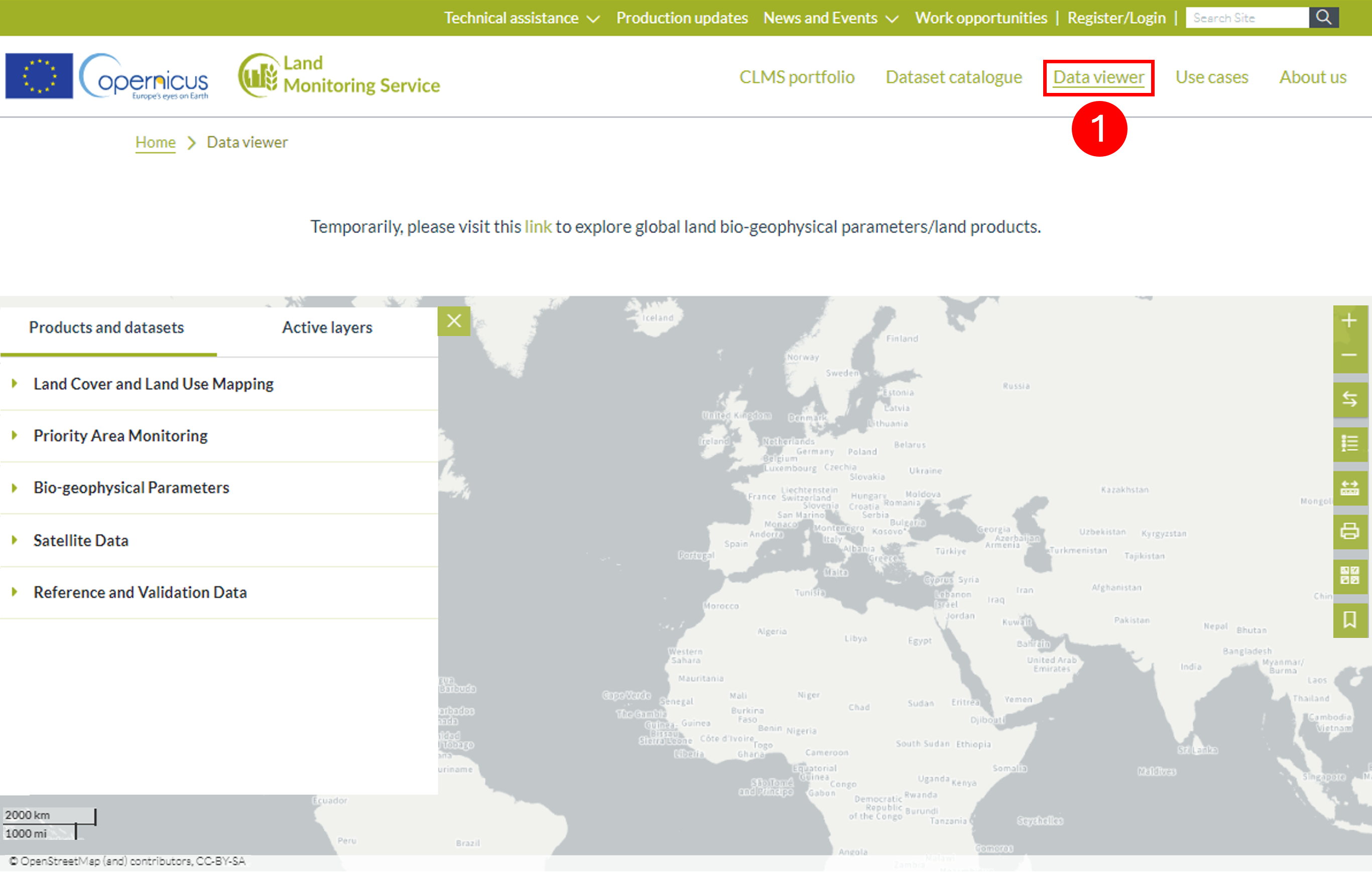
Fig. 2.1.7 – CLMS website - Data viewer

By clicking on Use Cases (1) (Fig. 2.1.8) the page that will open will be set to show the Browse Use Cases catalogue tab (2) by default. In the top part of this tab, we have a highlight of the latest use case.

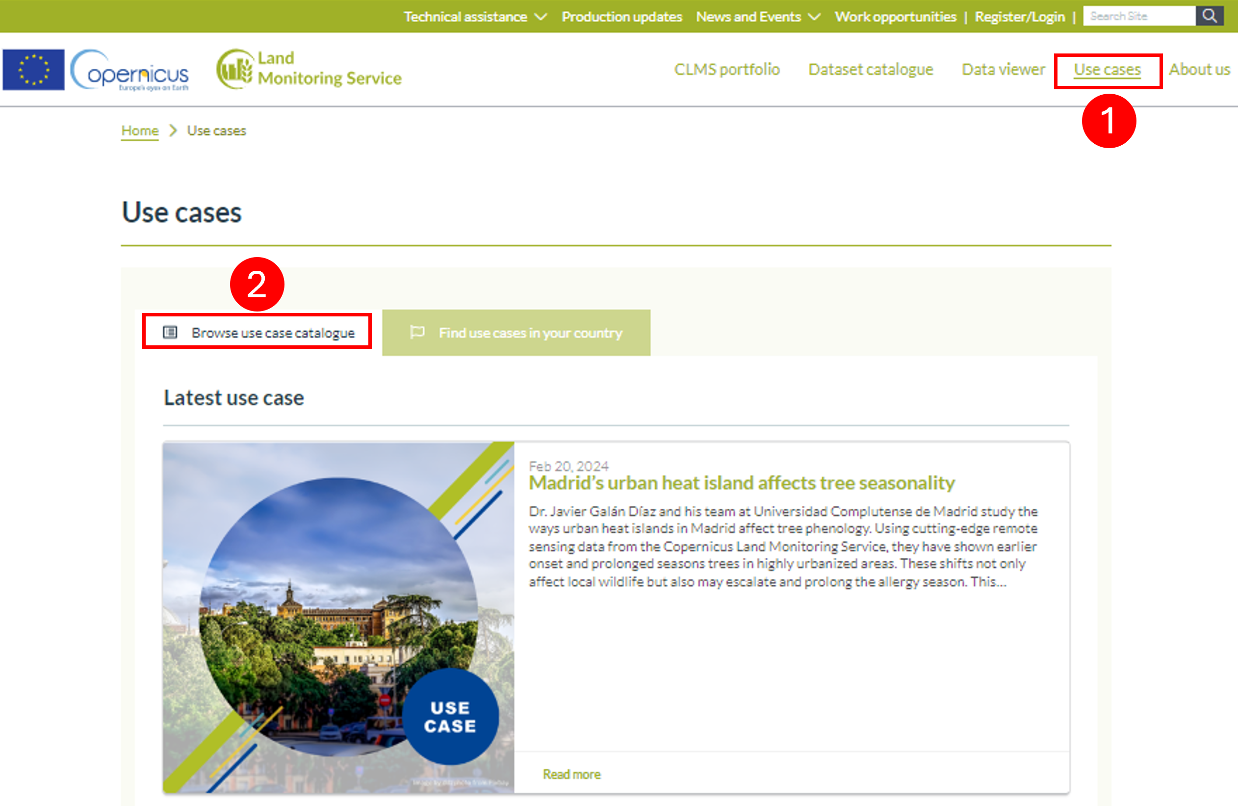
Fig. 2.1.8 – CLMS website - Use cases pt.1

Scrolling down in this tab we have a list of all activations (Fig. 2.1.9) and we can browse them using the search bar (1). There are many activations and some may not be shown directly on the page, if the activation we are looking for is not shown it is possible to move between the other activations using the arrows and/or page reference (2) at the end of the activations list. It is also possible to submit your own use cases by clicking on Submit your use case (3) and filling out a form.

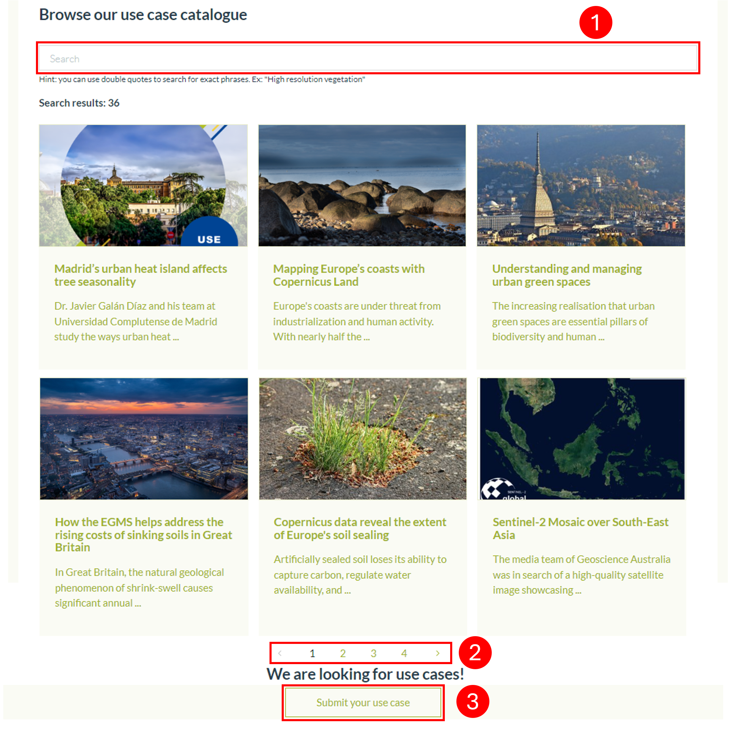
Fig. 2.1.9 – CLMS website - Use cases pt.2

From the top of the Use Cases page (Fig. 2.1.10) , we can open the second tab which is the Find Use Cases in your Country tab (1). From there you can use the interactive map (2) to look for use cases in a specific country.

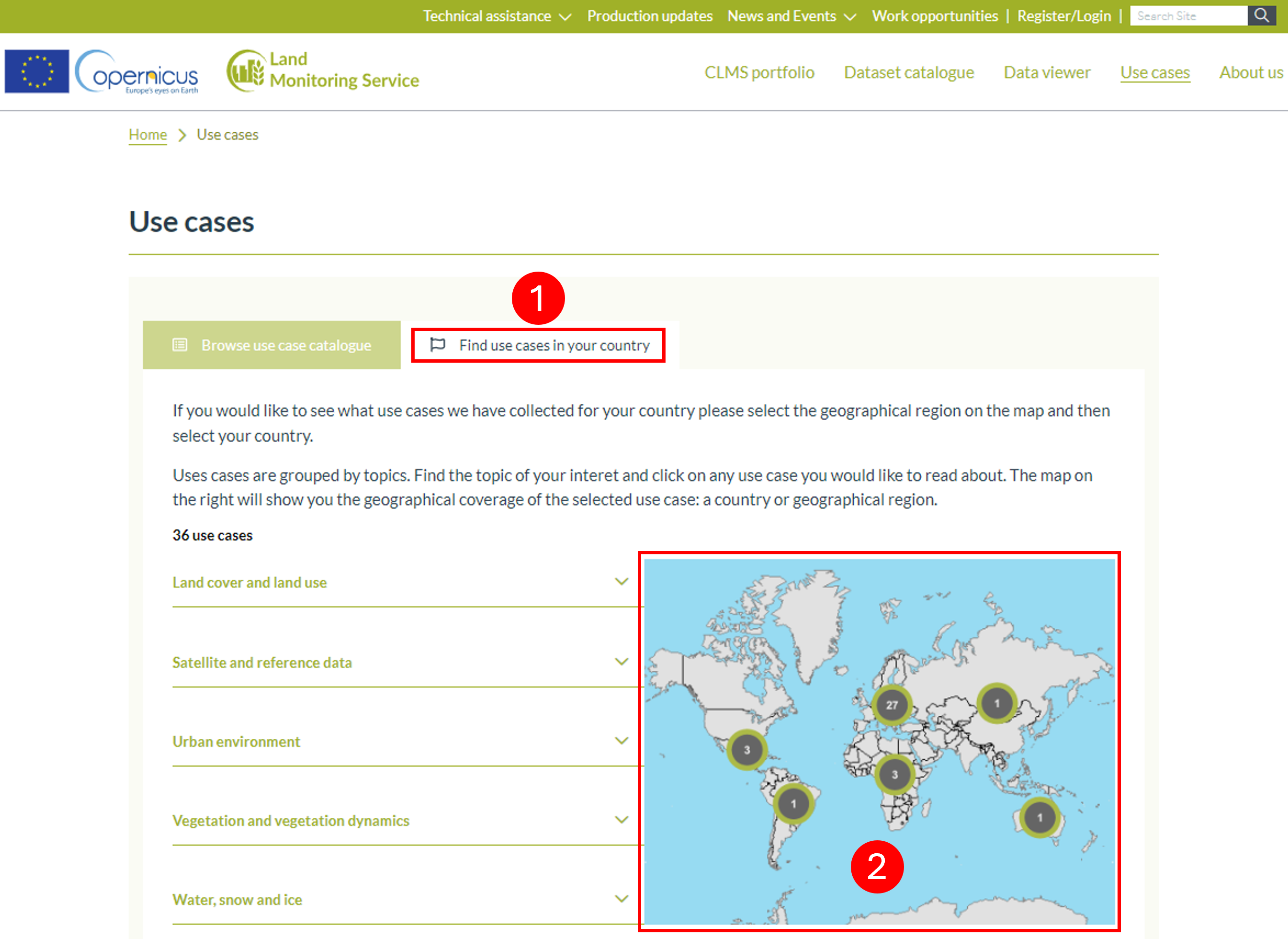
Fig. 2.1.10 – CLMS website - Use cases pt.3

The last page that we can reach from the main menu will group information about the CLMS (Fig. 2.1.11) . This page can be reached by clicking on About Us (1). Here there is information about what CLMS is and what it does. Ultimately there is the possibility to contact the helpdesk to seek answers to questions that do not find one on the website.

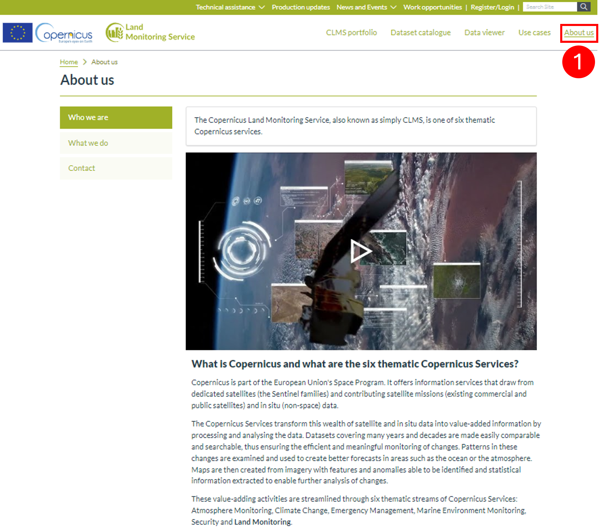
Fig. 2.1.11 – CLMS website - About us

2.1.1. The CORINE Land Cover layer

Among the CLMS products, the CORINE Land Cover (CLC) layer is of great importance for manifold applications. The CORINE (Coordination of Information on the Environment) programme is a component of the CLMS and a European effort to develop a standardized methodology for producing continent-scale land cover, biotope, and air quality maps. Specifically, the CORINE Land Cover product offers a pan-European land cover and land use inventory with 44 thematic classes. All products are free of charge and can be used for any purpose. It is updated every six years, with its last version in 2018; the 2024 reference year update is scheduled for publication in the first quarter of 2026. In the following sections, we propose an exercise based on the exploitation of the CLC layer. The exercise involves the following steps:

• download the CLC layer
• import the CLC layer in QGIS
• apply a standard symbology
• clip the layer to the extent of the flooded area

2.1.1.1. CLMS Map Viewer

Click on Data Viewer . You will be redirected to the data viewer application (Fig. 2.1.1.1) . Inside the Products and Dataset menu (1) a list of all products is shown and we can activate them, in this example, only the CORINE Land Cover dataset has been activated (2) between all CLC products only the CLC relative to 2018 has been activated (3). Active layers are shown in the map (4) and can be seen in the Active layers menu (5). A list of all buttons on the right of the screen is reported here:

• Zoom in and Zoom out (6): allow to zoom in and out the map;
• Swipe (7): from here you can set a Leading Layer and a Trailing Layer;
• Legend (8): shows the legend of all active layers;
• Measurement (9): allows you to compute measurement on the map in terms of distance and area and also allows you to know the coordinates of every point on the map where you place your mouse;
• Print (10): allows you to download Layout or Maps
• Basemap gallery (11): allows you to change the base map;
• Layer info (12): allows you to click on the map to get pixel information
• Bookmark (13): allows you to bookmark the current map in order to retrieve it later

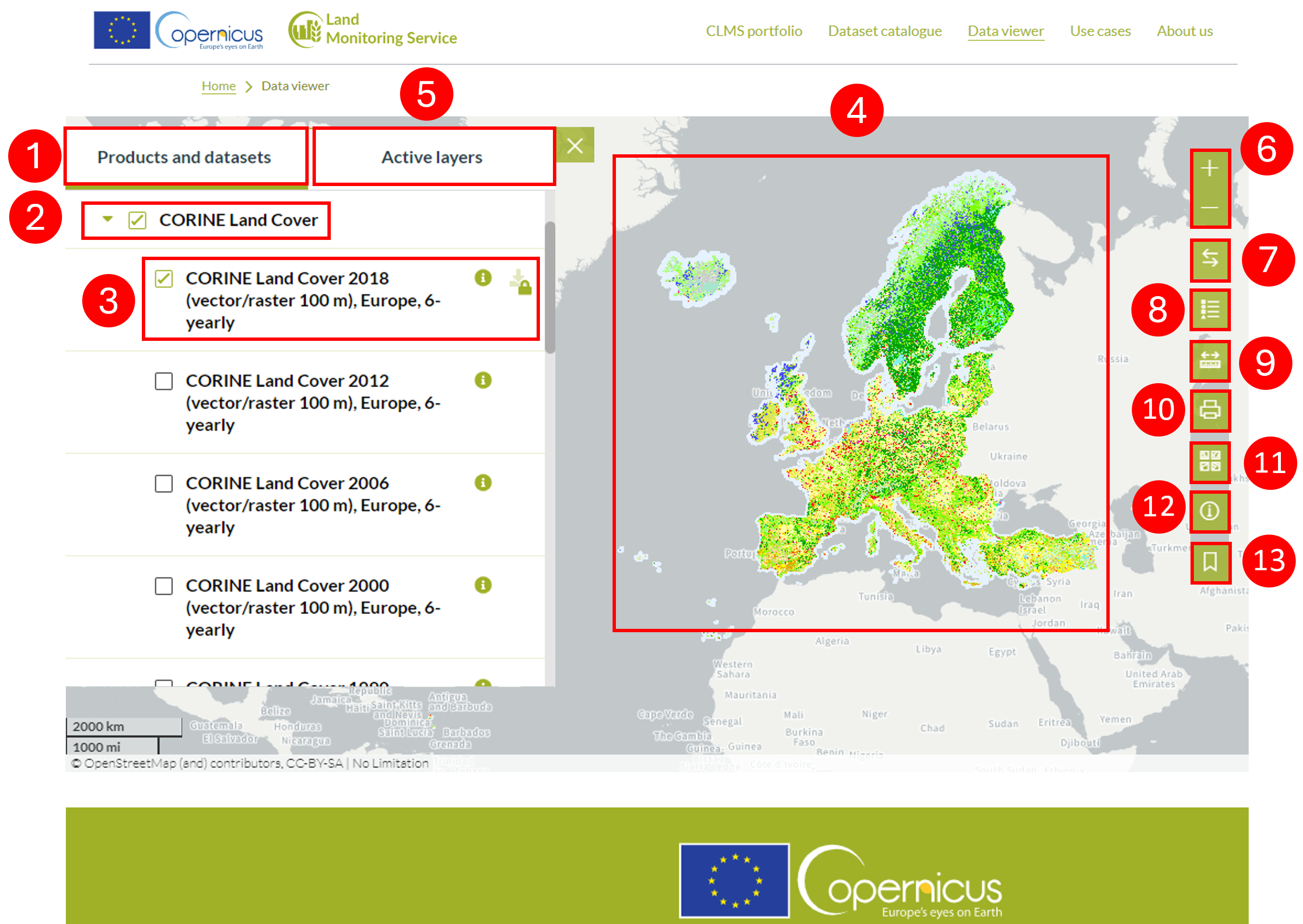
Fig. 2.1.1.1 – LMS data viewer

Click on this link for Downloading the CORINE Land Cover 2018 layer. This link will lead you to the web page illustrated in (Fig. 2.1.1.2), to start downloading the land cover layer after accessing the website. Firstly, click on Download (1), and a new window, asking you to log in, will pop up (2). Follow the link to create an EU account (3). A login is required for data downloading from CLMS.

Warning

you might need to be over 18 to be able to create an account.

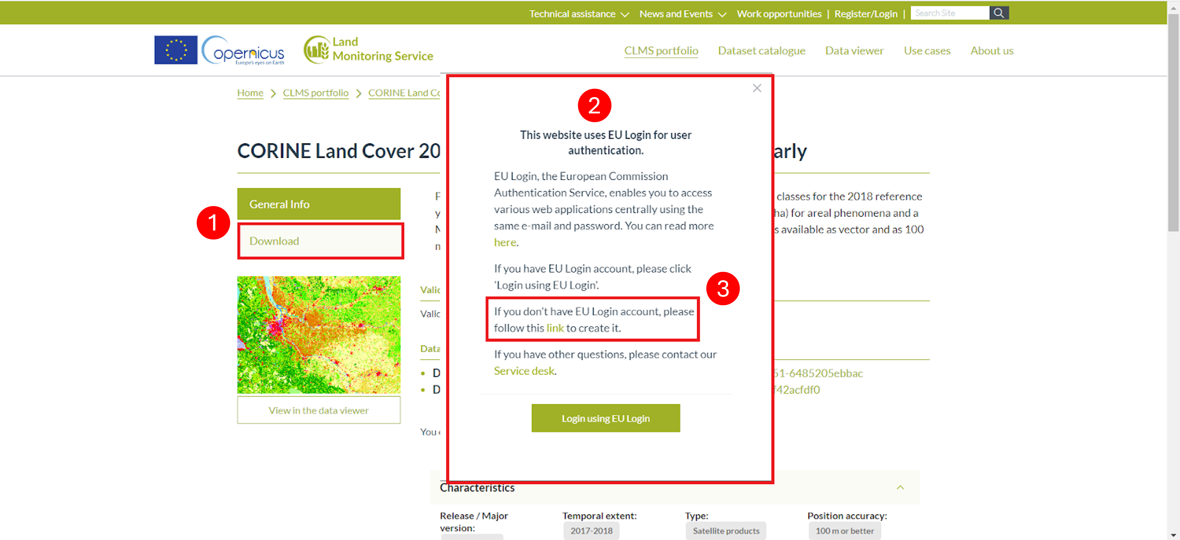
Fig. 2.1.1.2 – User authentication

After login, you will notice your username is written in the top bar (1) as illustrated in (Fig. 2.1.1.3) , together with the cart that you can fill in with the data that you are interested in (2)**. You can visualize the land cover layer and select the area of interest: click on Go to download by area (3). The selection of a specific area of interest has the advantage of occupying less storage space while requiring less computational time when dealing with the data in QGIS.

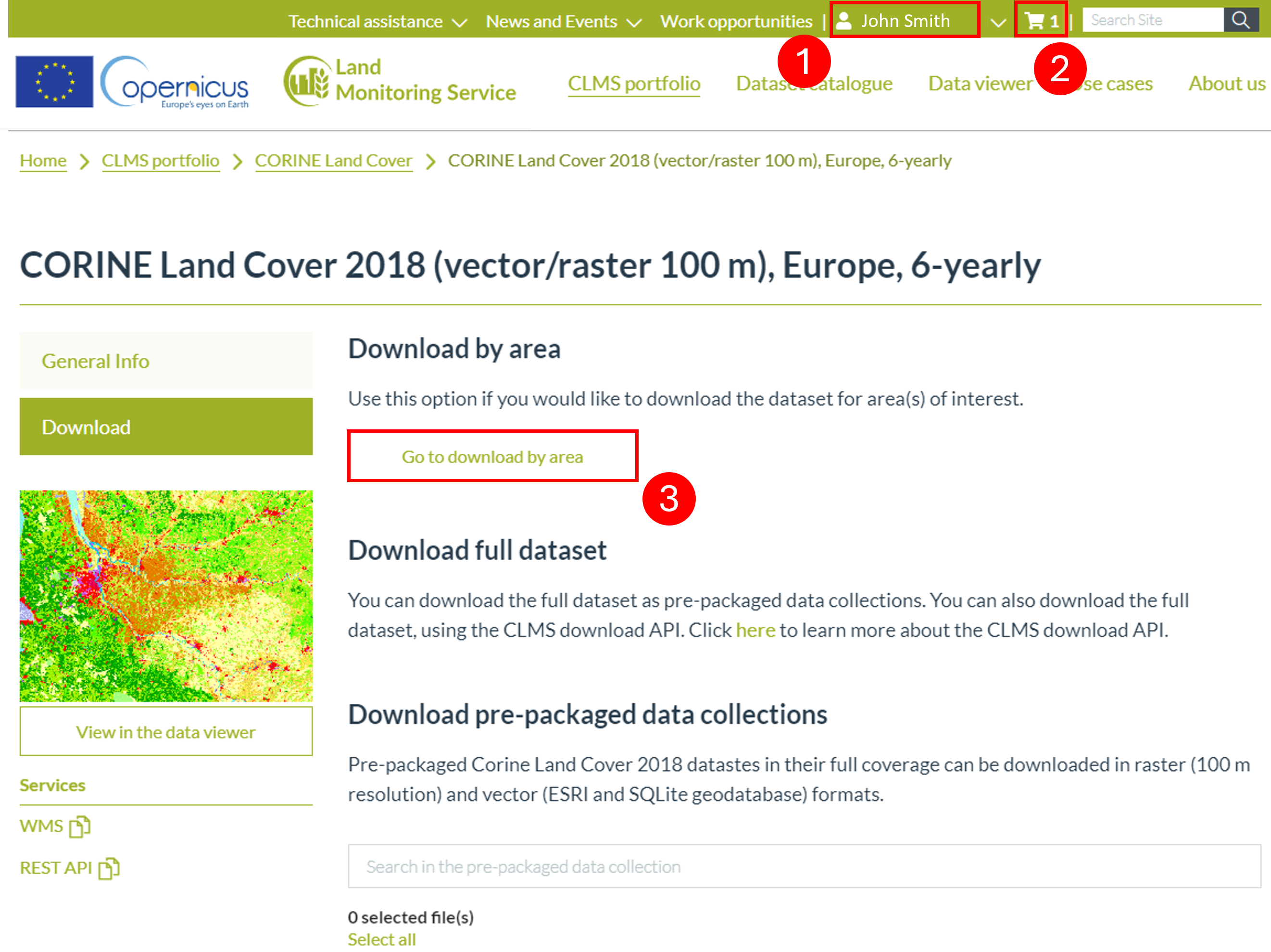
Fig. 2.1.1.3 – LMS Interface after login

After a click on Go to download by area, you can select the area of interest by clicking on the icon with the dotted line and the mouse arrow (1) (Fig. 2.1.1.4) , and then selecting Draw a rectangle on the map (2). Click on a point on the map and drag your mouse. A black rectangle will appear. Be careful to include the area of interest. Now release it (3). Now click on the download icon (4), and your selected product will be added to the cart. Click on the cart icon (5).

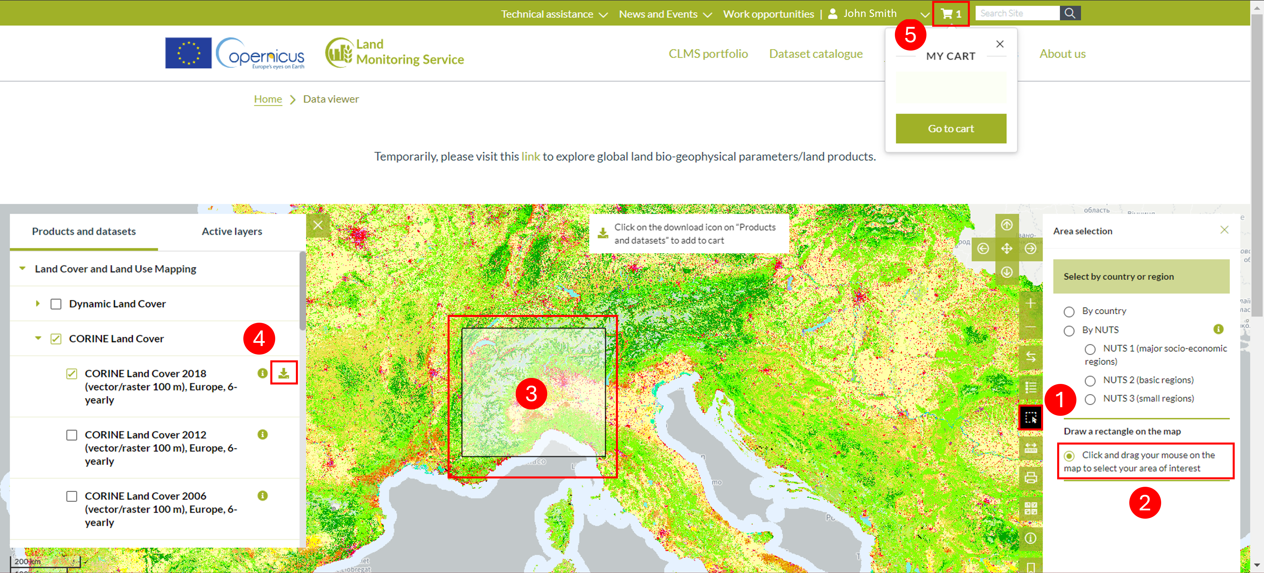
Fig. 2.1.1.4 – Download Corine land cover for the area of interest part 1

From the Cart (Fig. 2.1.1.5) you will see all your products, in this case, we placed only product one in the cart. Set the Type as RASTER (1) and the Projection to EPSG:4326 (Source system of the dataset) (2), once done, click on Process Download Request (3), after a few minutes you will receive an email containing a link to start your download.

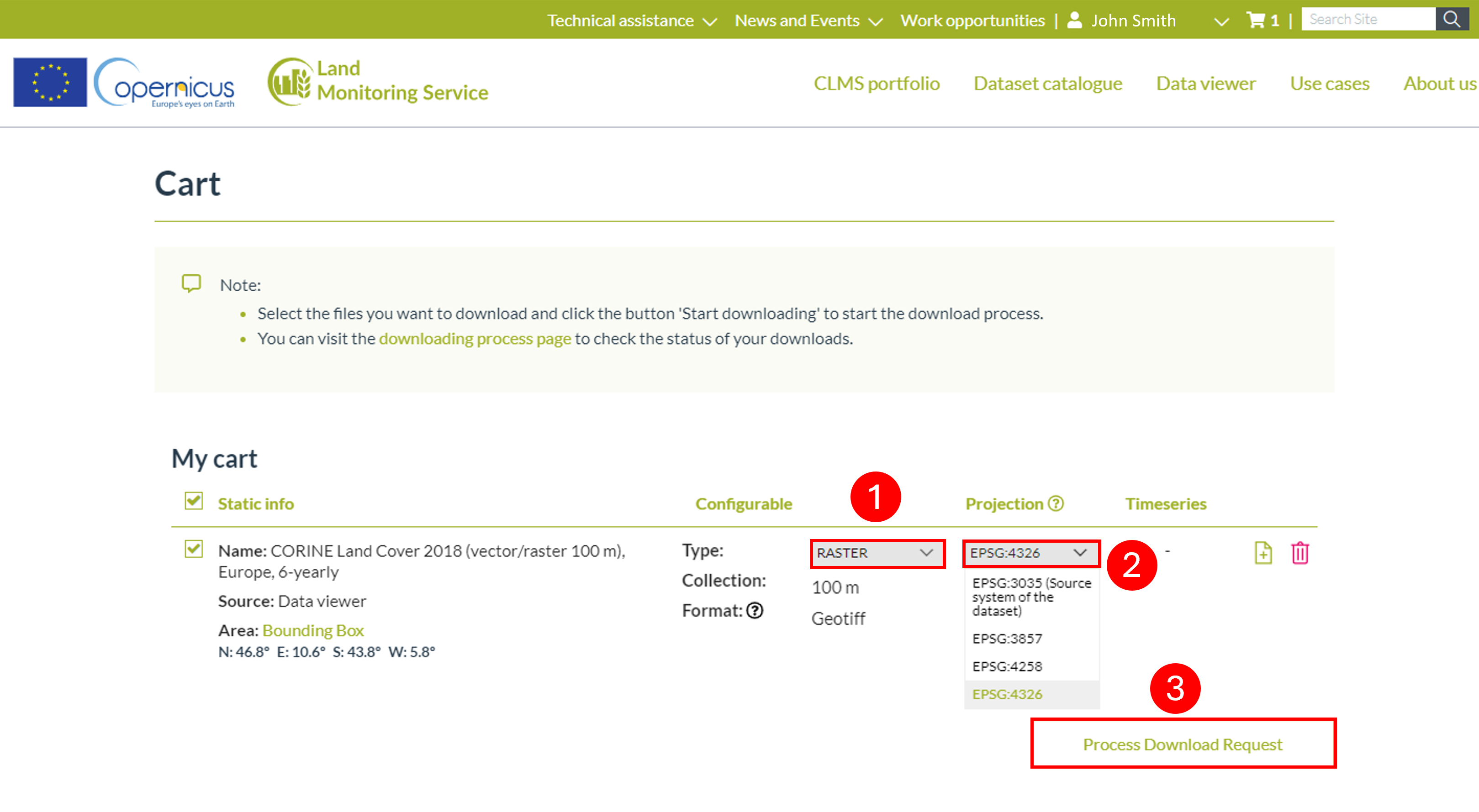
Fig. 2.1.1.5 – Download Corine land cover for the area of interest part 2

2.1.2. Importing CORINE Land Cover Layer in QGIS

The downloaded data are raster data, so we can add them in QGIS as seen in Chapter (421 add link). As shown in (Fig. 2.1.2.1) , click on Layer (1), then Add Layer (2) and choose Add Raster Layer (3). From the Data Source Manager click on the three-dotted button (4), and look for the “.tif” file in your folders (the file name is “U2018_CLC2018_V2020_20u1.tif”). You can now click on Add (5) and Close (6).

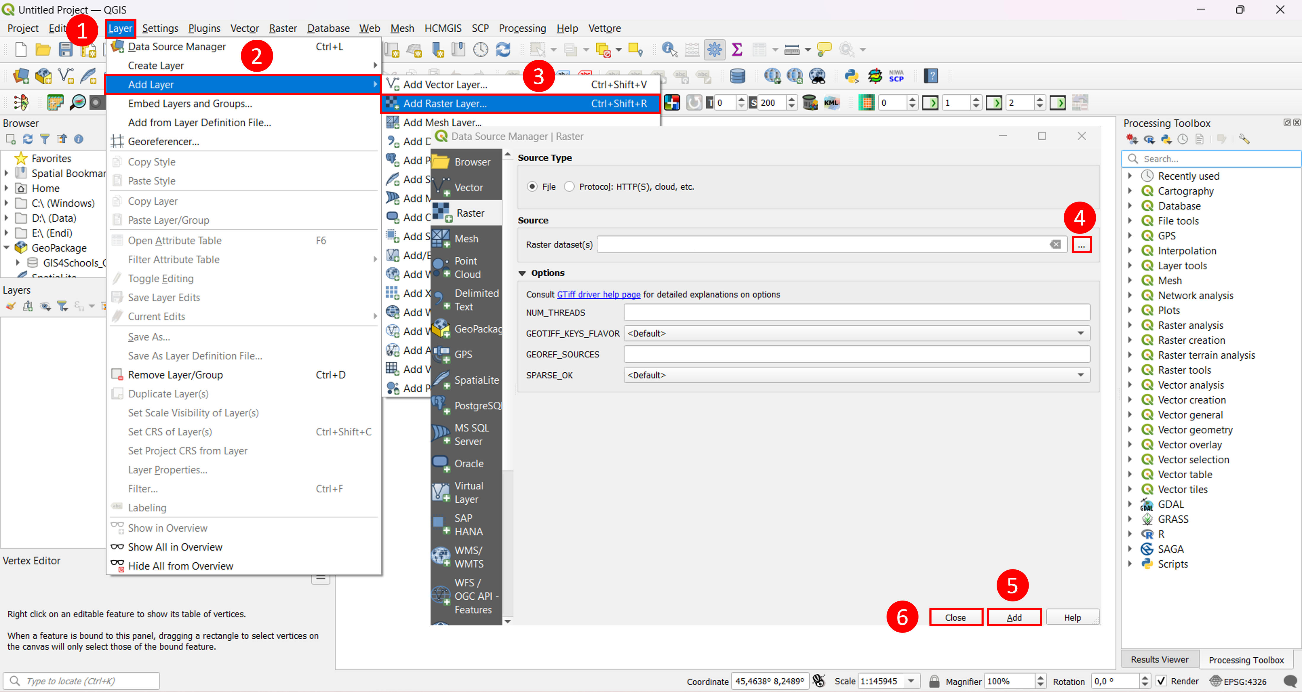
Fig. 2.1.2.1 – Import raster data in QGIS

2.1.2.1. Load Style

A file containing the style of the CLC layer has been downloaded as well, and it can be easily imported in QGIS as follows (Fig. 2.1.2.2) . First, right-click on the layer you have just imported in QGIS (1), go to Properties (2) and open the Symbology menu (3). In the bottom right corner click on Style (4) and select the Load Style… option (5). In the Database Styles Manager menu that will pop up, click on the three-dotted icon (6), the path to find your data should look like this: “…Results65791EEAU2018_CLC2018_V2020_20u1_raster100m_tiled_docInfoLegendRasterclc_legend_qgis_raster.qml” except for the first part where you need to find where the Results file has been saved and the product identifier that can be different. The .qml format is human-readable and can be easily edited using a text editor or within QGIS itself where it is used to store information about layers style. In general this file format is used to define layouts of the user interface like the position of images and buttons. Once you have imported the file, click on Load Style (7) and OK (8).

..note:: You can read more about .qml format here .

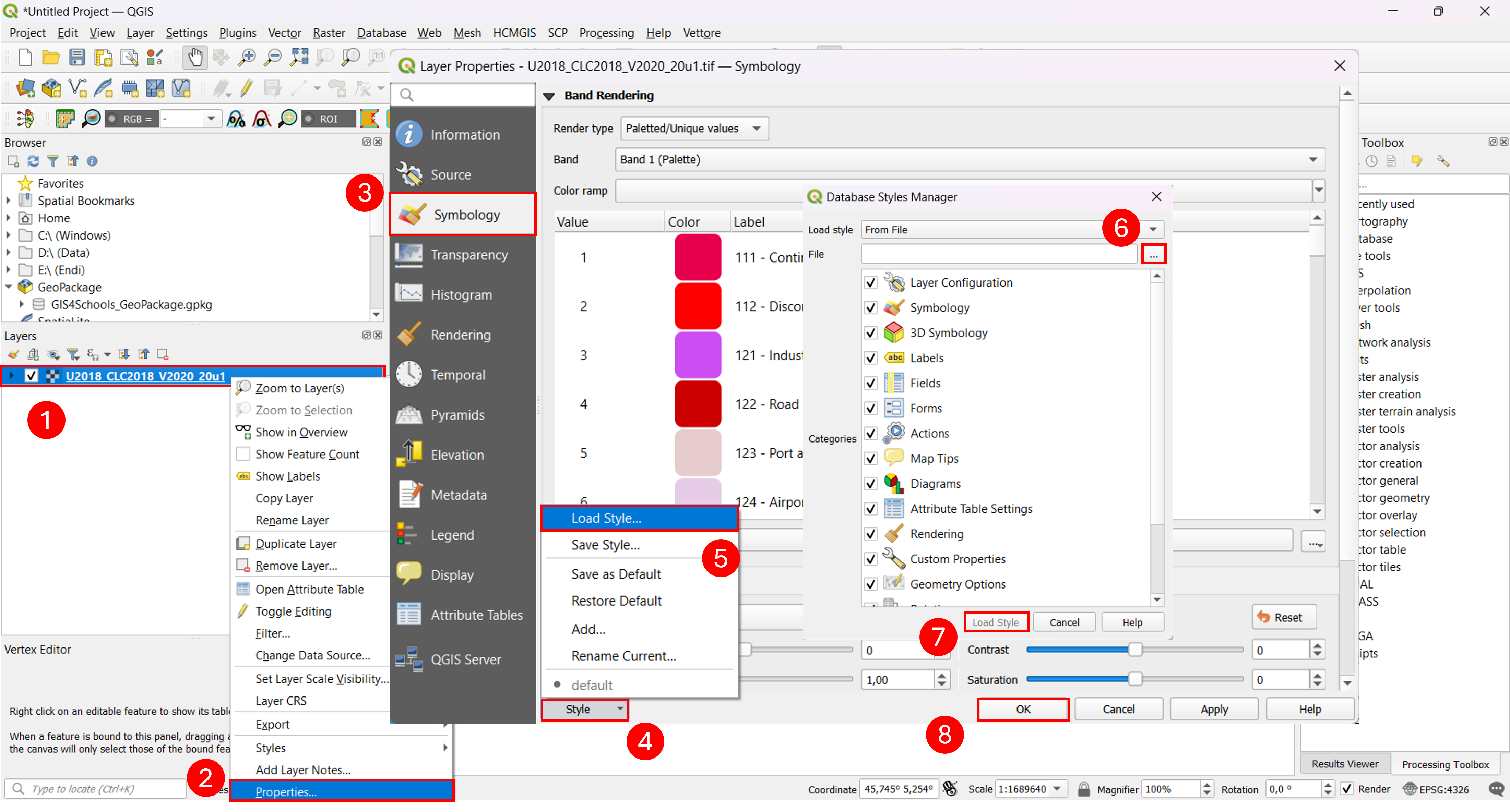
Fig. 2.1.2.2 – Load style

2.1.2.2. Flooded area land cover classes

In the next steps, we will do some basic preprocessing to our data by projecting the coordinate system and by limiting the land cover data to only the portion relevant to the study area using the Clip tool. This procedure is particularly useful to reduce the computational burden of managing data larger than your area of interest. You will also learn to copy and paste a style from one layer to another. With this technique, you will be able to spare time while working with data using the same styles.

Clip the Land Cover Layer to the area of interest

Import the area of interest (“EMSR468_AOI05_DEL_PRODUCT_areaOfInterestA_r1_v1”) and observed event (“EMSR468_AOI05_DEL_PRODUCT_observedEventA_r1_v1”) layers used in lecture 3 (add link). We will start by reprojecting the area of interest layer layer (Fig. 2.1.2.3). In the Processing Toolbox search bar type “Reproject layer” (1). Click on the Reproject layer tool (2) which will be under the Vector General group. Set “EMSR468_AOI05_DEL_PRODUCT_areaOfInterestA_r1_v1” as the Input layer of the tool (3). Under Target CRS click on the Select CRS icon (4), a new section of the tool will open up, from there type “WGS 84 / UTM zone 32N” into the Filter search bar (5). Click on the selected projection (WGS 84 / UTM zone 32N EPSG 32632) (6) and then on the blue arrow in order to go back to the previous tab (7). If everything was done in a correct way you should see the selected projection under Target CRS (8). Now proceed by choosing where to save your reprojected layer and by giving it a name (9), for the purpose of this lecture we will call it “AreaOfInterest_UTM”. Once done click on Run (10). Repeat this procedure by setting as Input layer the “EMSR468_AOI05_DEL_PRODUCT_observedEventA_r1_v1” layer, this second output will be called “ObservedEvent_UTM”.

..warning:: Make sure that both output files are saved with the .shp extension.

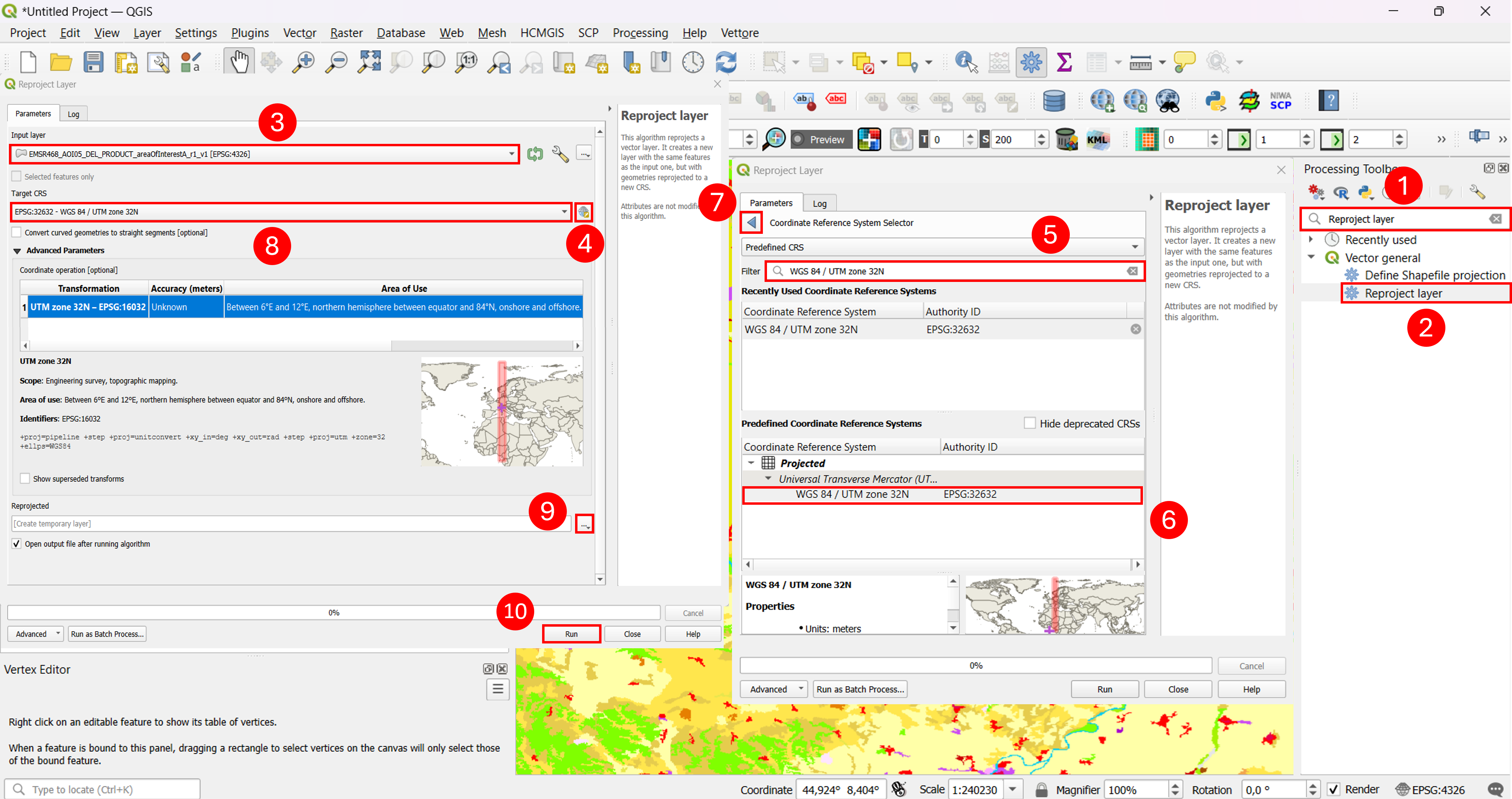
Fig. 2.1.2.3 – Reproject Vector Layers

We will now reproject the land cover layer. Click on Raster (1), Projection (2) and then select Warp (Reproject) (3). Set “U2018_CLC2018_V2020_20u1.tif” as the Input layer of the tool (4). Now we want to set Target CRS as “WGS 84 / UTM zone 32N EPSG 32632”, to do so you can click on the drop down menu (5), if you recently used this CRS it will appear in the menu allowing you to select it. Otherwise click on the Select CRS icon (6) and search for it in the same way as shown in Fig. 2.1.2.4 . Now proceed by choosing where to save your reprojected layer and by giving it a name (7), for the purpose of this lecture we will call it “LC_UTM”. Once done click on Run (8). ..warning:: Make sure that the output file is saved with the .tiff extension.

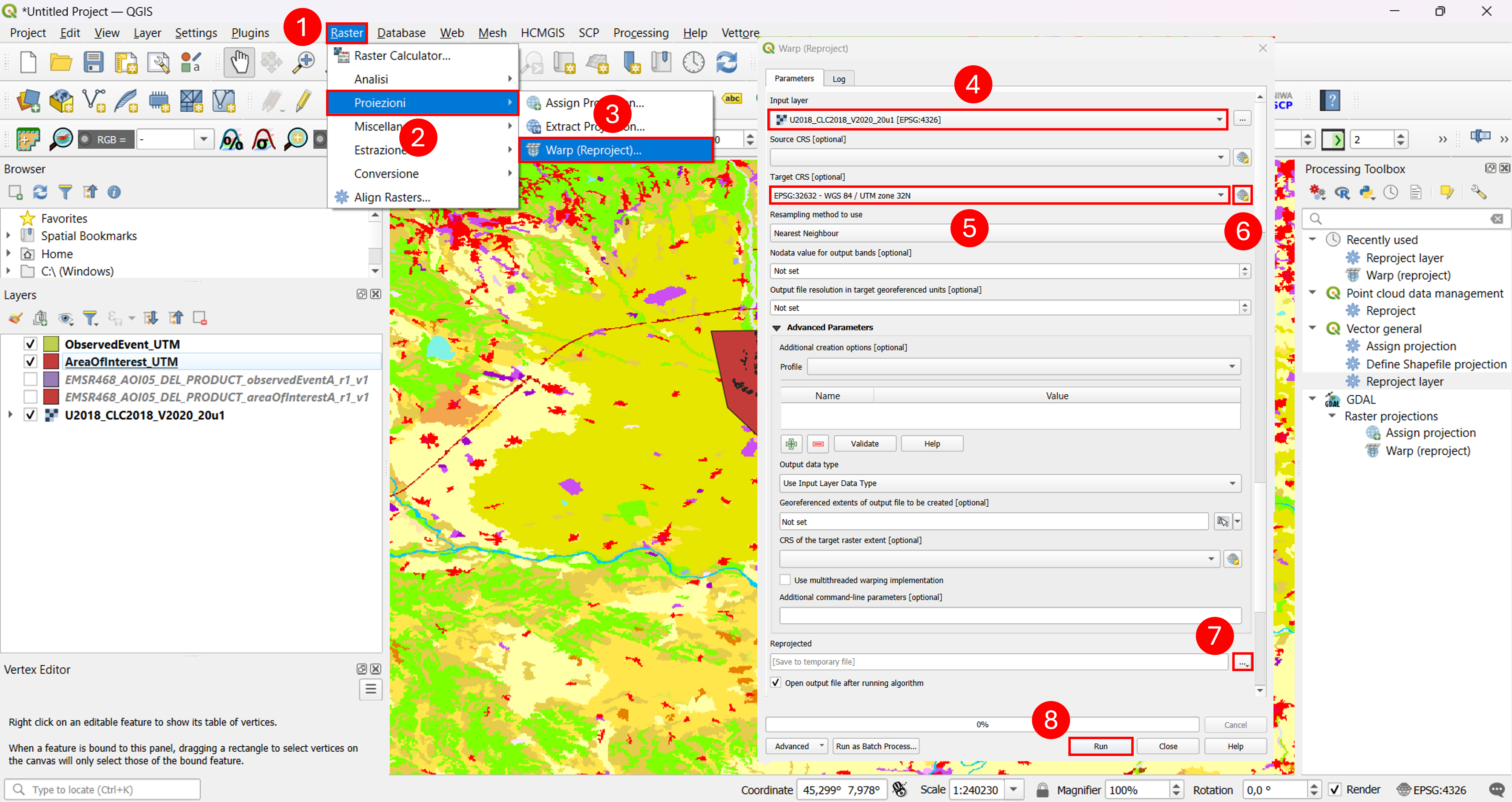
Fig. 2.1.2.4 – Reproject Raster Layers

Clip the Land Cover Layer to the area of interest

You can notice that the downloaded land cover data includes a way wider area than the one we are interested in. To tackle this issue, we can “cut out” the data to the portion of interest. Now we can proceed with the clipping procedure (Fig. 2.1.2.5) . Click on Raster (1) then on Extraction (2) and on Clip Raster by Mask Layer… (3). In the menu that appears, set the land cover layer as the Input layer (4) and the area of interest layer as the Mask layer (5). Once done, click on Run (6).

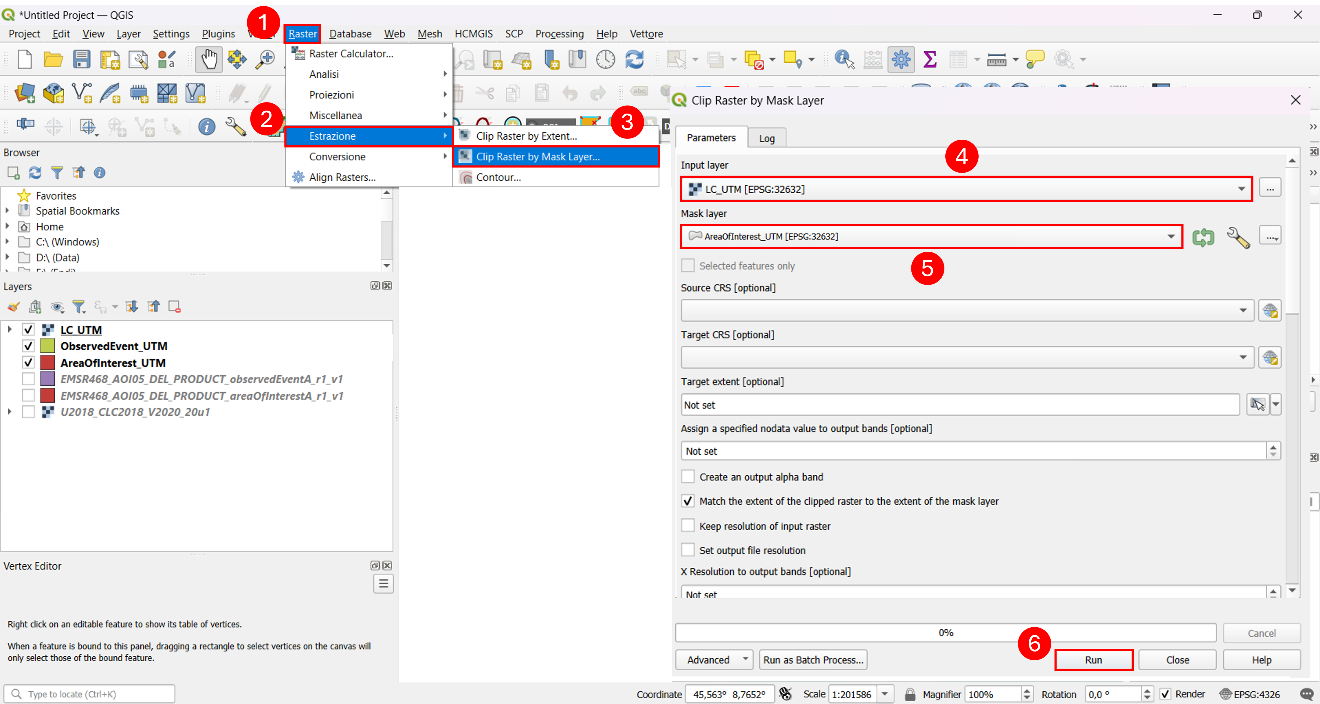
Fig. 2.1.2.5 – Clip data

Apply Style

After the previous steps, you should have lost the original layer style. To retrieve it, you can copy the style of another layer. To do so, right-click on the layer you want to take the style from (“U2018_CLC2018_V2020_20u1”) (1) (Fig. 2.1.2.6) , select Style (2), Copy Style (3) and click on All Style Categories (4), as displayed in (Fig. 5.1.2.2.2b).

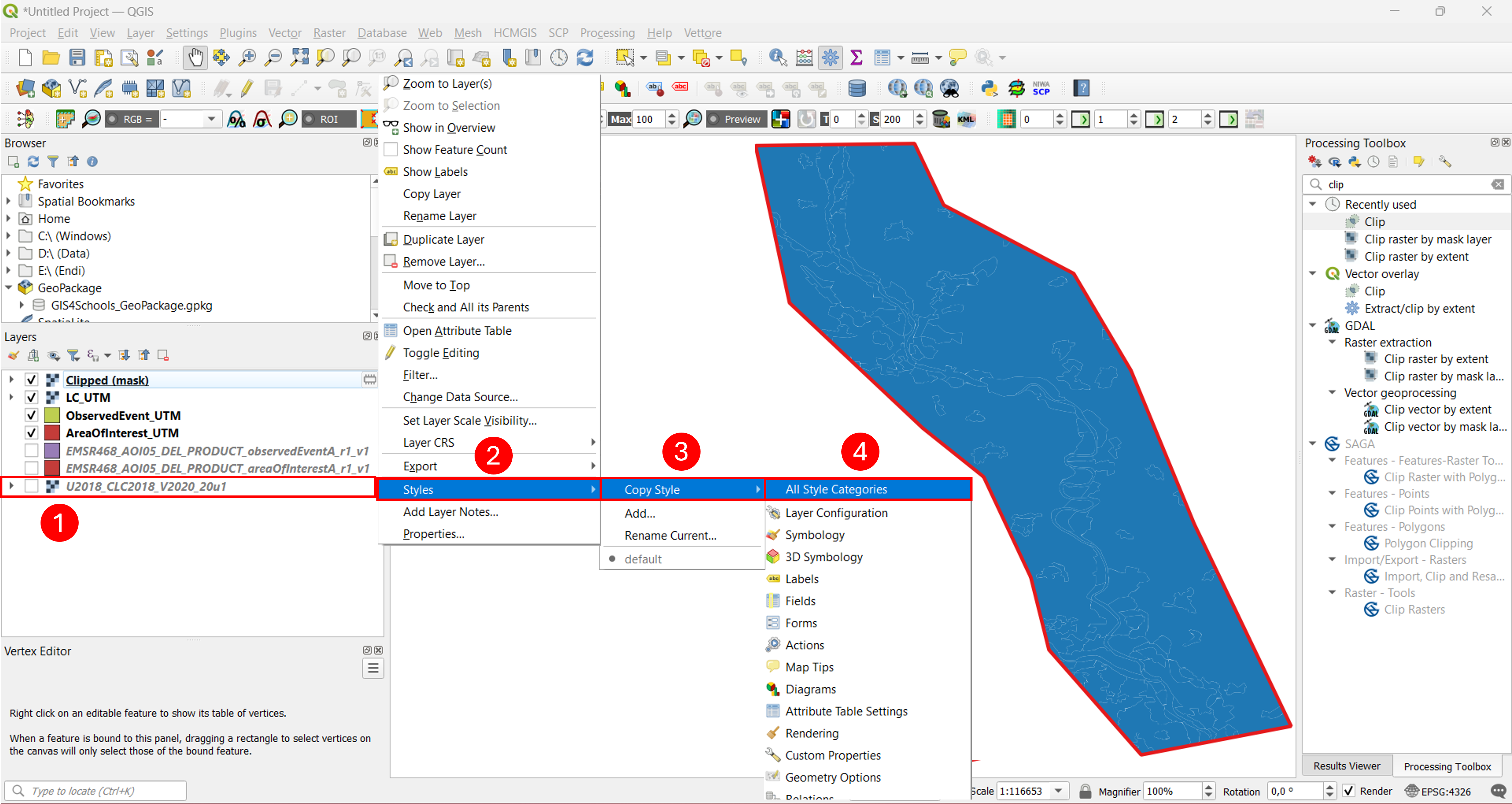
Fig. 2.1.2.6 – Copy style

Now we need to paste the style we just copied to our clipped layer (Fig. 2.1.2.7) . Right-click on the clipped layer (1), select Style (2), Paste Style (3) and click on All Style Categories (4).

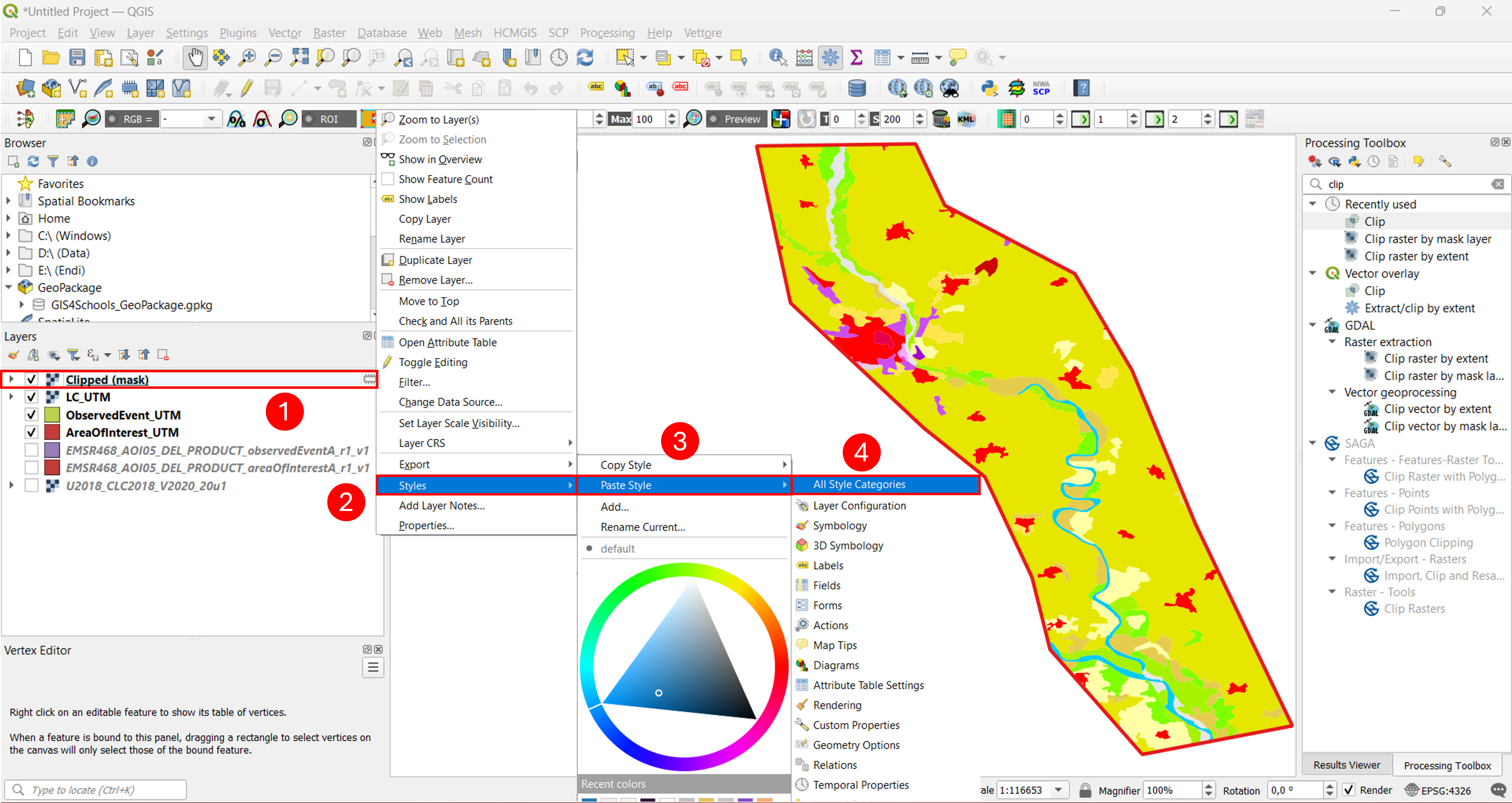
Fig. 2.1.2.7 – Paste style

Save Layer As you can see, when we clipped the layer, we did not save it, this is also denoted by the icon that appears on the left of temporary layers (Fig. 2.1.2.8) . Since the layer is temporary it will be lost once QGIS will be closed. This can be a very useful feature in case we do not need to use that layer anymore but it is not our case. In order to save the Clipped layer we can right click on it (1), go on Export (2), Save As… (3). Now proceed by choosing where to save your layer and by giving it a name (4), for the purpose of this lecture we will call it “LC_UTM_Clipped”. Once done click on OK (5).

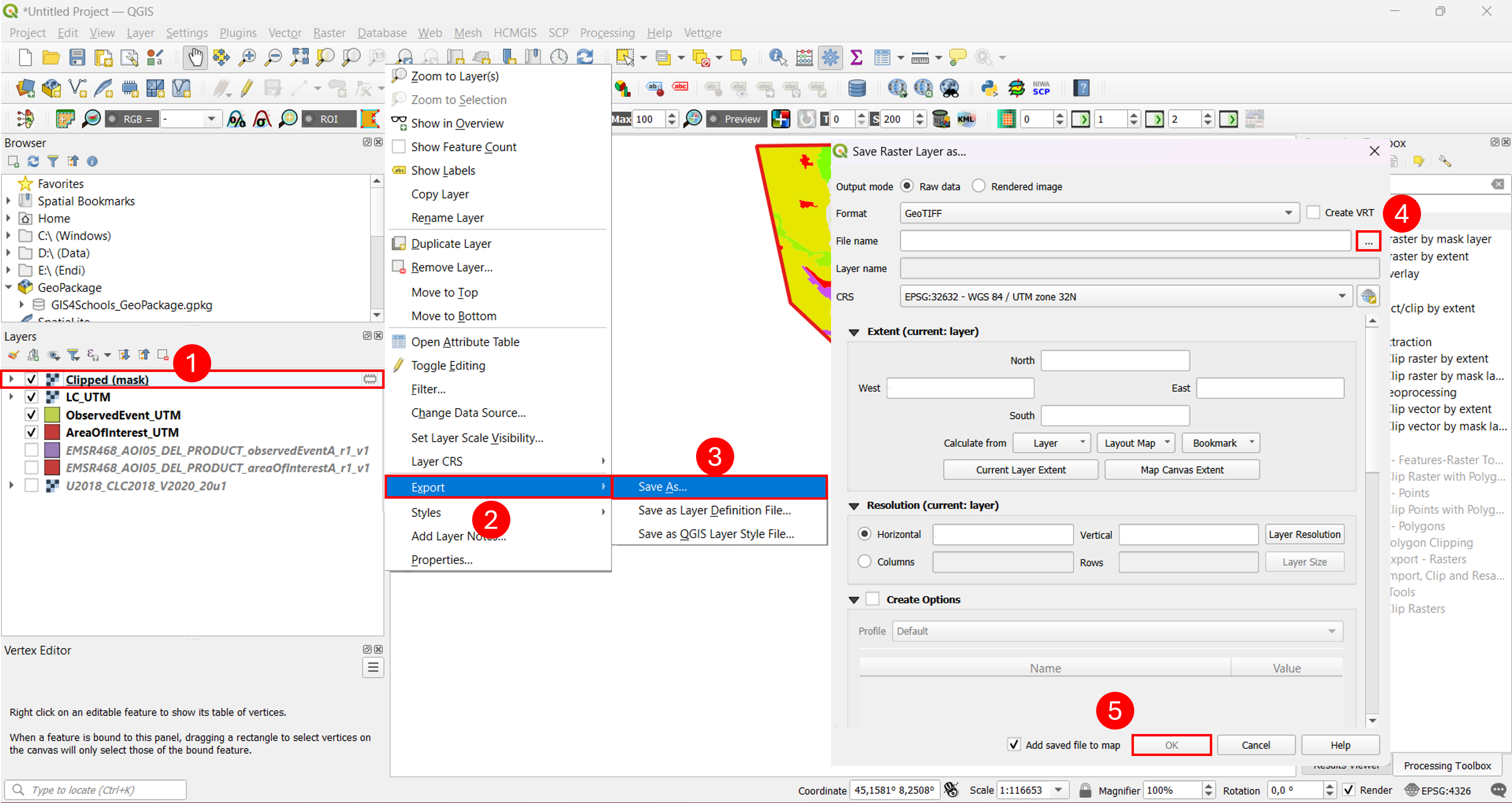
Fig. 2.1.2.8 – Paste style