1.1. What are Geographic Information Systems?
A geographic information system (GIS) is a system that can be used to analyze, manipulate, integrate, and map different data types. Through it, it is also possible to manage georeferenced data. GIS is used for a wide range of applications that span from visualizing bird biodiversity maps using data gathered through citizen science to monitoring a flooding event. “A GIS is an integrated system of computer hardware, software, and trained personnel linking topographic, demographic, utility, facility, image and other resource data that is geographically referenced” US National Aeronautics and Space Administration (NASA) GIS are composed of several elements (Fig. 1.1.1):
- Data: Digital or analog information linking attributes with geographic locations
- Methods: Mathematical models and analytic techniques to manipulate spatial data
- Software: Written instructions (source code) that can be read by computers to implement methods
- Hardware: Equipment to support the activities needed for spatial data collection, storage, processing, analysis, and display
- People: Trained GIS professionals and end-users
- Network: Provides connections among all the GIS components

Fig. 1.1.1 – GIS elements
The suggested first step to novice users for learning GIS is through desktop GIS applications (Fig. 1.1.2) . Desktop GIS are software applications, running on workstations and laptops, allowing users to access information using spatial logic and methods, to modify or create from scratch spatial data, and to visualise the results as a map. They also Provide graphical user interfaces and facilitate cooperation among users through the adoption of standard formats (exchange spatial data files but also complete mapping projects and analysis procedures). They also offer support for network connection enabling access to online GIS resources. There exist many models of software development and distribution such as freeware, shareware, FOSS etc. and, being users, it is fundamental to know the difference between them. Here we will see two of the most common:
- A proprietary GIS software is copyrighted and has limits against distribution and modification that are imposed by its owner. Generally, the use of proprietary GIS software is allowed to end-users with payment licenses.
- A FOSS (free and open-source software) GIS is released under a license in which the copyright holder grants users the rights to use, study, change, and distribute the software to anyone and for any purpose. These rights are guaranteed to any users free of charge
Fig. 1.1.2 – Proprietary and free and open-source software
1.1.1. Coordinate Reference System
Geographic location is the element that distinguishes spatial data from all other types of information, so methods for specifying locations on the Earth’s surface are essential to GIS. Many techniques have been developed over the centuries to define locations, but only thanks to GIS it has become possible to automatically switch from one to another. To understand GIS and spatial data we must have in mind what is a coordinate reference system (CRS) and how they are established for the Earth. In order to define what is a coordinate reference system (CRS) we first need to talk about Coordinates and Datum.
Coordinates are a sequence of values representing a location and form the basis of a coordinate system which is a sequence of coordinate axes where the unit of measurement is being specified. A datum is a mathematical model specifying the relationship through a coordinate system and the Earth, it is a modeled version of the Earth’s surface. The best description of Earth’s shape is provided by the geoid which results from complex physical models and describes the surface of equal gravity formed by the oceans, and its extension under the continents. For traditional GIS application, the geoid can be approximated using a sphere or, better, an ellipsoid of rotation. The ellipsoid known as WGS84 (the World Geodetic System of 1984) is currently the most widely accepted global geodetic datum and it is the one used, for example, by the Global Positioning System (GPS) When a coordinate system is complemented with a datum, we get a coordinate reference system (CRS). Each point in the geographic coordinate system has two coordinate values: latitude (φ) and longitude (𝜆) (Fig. 1.1.1.1) : The Latitude is the angle formed by the intersection of a line perpendicular to the Earth’s reference surface at the point, and the Equator. Lines of constant latitude are also called “parallels” The Longitude is the angle between the plane crossing the North and South poles and a reference plane. Lines of constant longitude are termed “meridians” and the reference plane is identified by the prime meridian (recognized with the meridian passing through Greenwich, UK)

Fig. 1.1.1.1 – Schematic of geographic coordinates system. The geographic coordinates of point p are defined by the angles φ (latitude) and λ (longitude)
1.1.1.1. Projection
We define a projection as a method used to translate data from a three-dimensional surface of the Earth to a 2D representation. This process brings with it some distortions as there is no way of maintaining the scale of areas, distances, angles and directions at the same time. There exist many projections (Fig. 1.1.1.2) but, usually, when we look at world maps, we come in contact with maps using the Mercator projections. This kind of projection is especially used for navigation charts since straight lines drawn on it are lines of constant bearing. Mercator projection is also a conformal projection which means that angles and shapes are preserved at the cost of losing the scale of the area. Check out http://thetruesize.com !
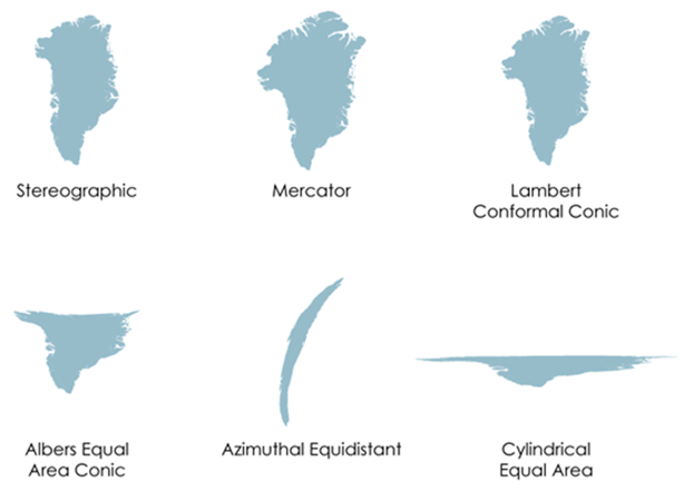
Fig. 1.1.1.2 – Distortions of Greenland area from different sample map projections. Source: https://www.axismaps.com
Digital catalogues Many CRS and projections have been developed and GIS allows converting spatial dataset between any CRS and projections. Digital catalogues containing encoded parameters (such as units, datums and projection formulas) of the different CRS is of primary importance to safely convert data from one CRS to another in an automatic way using GIS software The most popular catalogue is the European Petroleum Survey Group (EPSG) Geodetic Parameter Dataset which is a database of CRS information maintained by the International Association of Oil and Gas Producers Every CRS has a unique integer identifier (For example, the EPSG code of WGS84 is 4326). For more information you can visit the EPSG .
1.1.2. GIS Data
GIS data can be collected in different ways such as map digitization, direct survey, aerial survey and satellite measurements, each method with its pros and cons. Models are then used for encoding geographic information in a computer environment. GIS data models are a set of constructs and abstractions for describing and representing geographic entities in a digital system, they reshape geographic entities into discrete objects (vector models) or continuous surfaces (raster models) and fit both numerical and/or textual attributes with coordinates into computer files. The structure of these models is independent of specific data items and, in most cases, of the GIS application that is used to manipulate them. Also, GIS data models are often interchangeable so that the same geographic entity or phenomenon may be represented by different models, we will see interchangeability examples in future chapters.
..note:: The right data model to use strictly depends on the specific application (no single data model is the best for all circumstances)
The two main types of spatial data used in GIS are represented by Raster and Vector data.
1.1.2.1. Raster Data
Through Raster data we represent the world as a regular grid or matrix of pixels (Fig. 1.1.2.1). Each cell location is defined by the type of raster coordinate system, the coordinate of the raster origin, which is usually placed in the upper or lower left corner and the cell size. The resolution of a raster dictates the level of detail it can capture. With this representation we can depict both discrete phenomena like land cover or administrative boundaries and continuous ones, like elevation, temperature, land cover class, soil type etc. Operations on raster data are (generally) computationally fast due to the regular matrix format that can be easily handled by GIS software, that is why raster data are particularly suitable for mapping large portions of the Earth surface.

Fig. 1.1.2.1 – Raster Data
1.1.2.2. Vector Data
With a vector representation, real world features are represented using three geometric features, points, lines and polygons (Fig. 1.1.2.2). Points define the foundation of this representation and their position is given by a set of coordinates while lines and Polygons consist of interconnected points. These three features can represent different real world features depending on the scale of the map, for example a road can be represented with a line in a small scale map or with a polygon in a large scale one. Usually vector data are provided with an attribute table where each attribute of a feature, such as text, dates and times, is stored in a different column. Vector data provide a sharp and scalable representation of geographic entities with almost no loss of portraying accuracy because entities boundaries are outlined directly by their coordinate values GIS provides many drawing functionalities to manually edit and styling vector data on maps. The higher the number of vertices and attributes the better is the level of detail provided by the vector data while the data file dimension increases. Mathematical operations on vector data are generally computationally slower than raster data due to the sparse or irregular object format to be handled by GIS software that is why vector data are particularly suitable for high-detail cartographic applications focusing on a finite number of discrete objects or involving confined geographic areas.
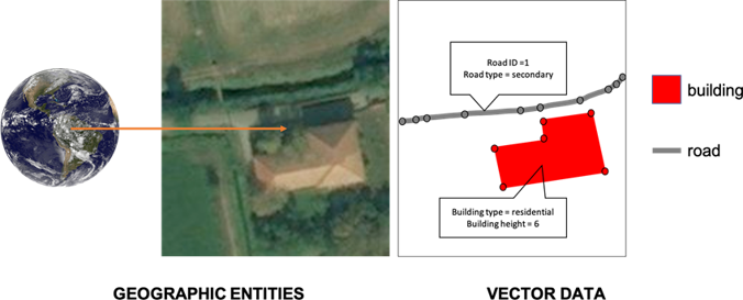
Fig. 1.1.2.2 – Vector Data