4.1. Visualization of GHSL-JRC population data in QGIS
In this lecture we need to import into QGIS the following layers:
- GHS_POP_E2020_GLOBE_R2023A_4326_3ss_V1_0_R5_C19.tif
- ObservedEvent_UTM
- AreaOfInterest_UTM
The first one has been downloaded in lecture 6 while the second and third one have been obtained in lecture 5 .
4.1.1. Data preprocessing
The first thing we will do is to reproject the “GHS_POP_E2020_GLOBE_R2023A_4326_3ss_V1_0_R5_C19.tif” (Fig. 4.1.1.1) . Click on Raster (1), Projection (2) and then select Warp (Reproject) (3). Set “GHS_POP_E2020_GLOBE_R2023A_4326_3ss_V1_0_R5_C19.tif” as the Input layer of the tool (4). Now we want to set Target CRS as “WGS 84 / UTM zone 32N EPSG 32632”, to do so you can click on the drop down menu (5), if you recently used this CRS it will appear in the menu allowing you to select it. Otherwise click on the Select CRS icon (6) and search for it in the same way as shown in Fig. 2.1.2.3 . Once done click on Run (7). .. warning:: Make sure that the output file is saved with the .tiff extension
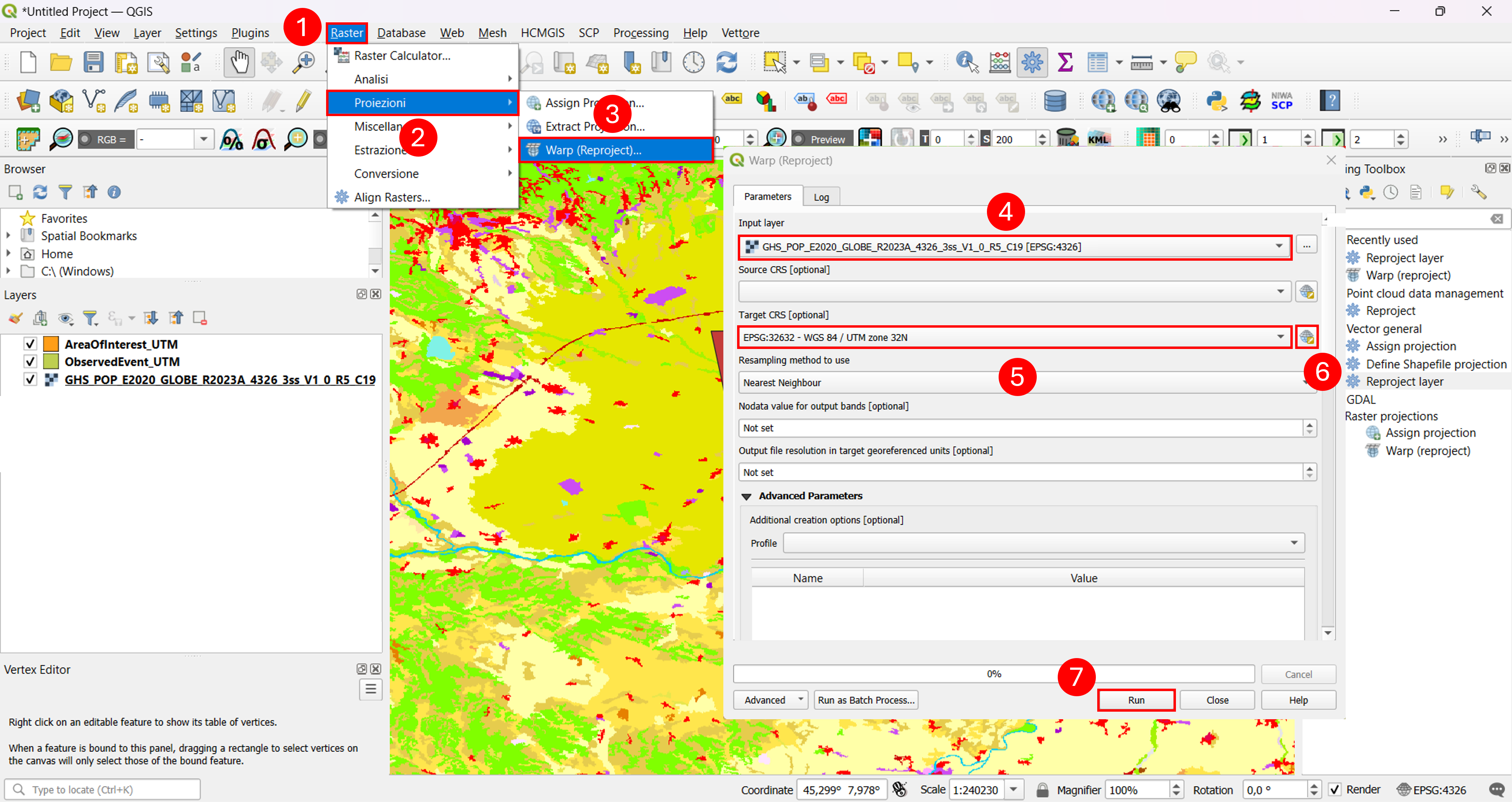
Fig. 4.1.1.1 – Reproject Raster Layers
Due to their size, our data requires a high computational burden to be managed, and it will be better to clip them to our area of interest (Fig. 4.1.1.2) . In order to do so, click on Raster (1), Extraction (2), Clip Raster by Mask Layer… (3). From the menu that just opened choose as Input layer the layer that we want to clip (“Reprojected”) (4) and as Mask layer the layer corresponding to our area of interest (“AreaOfInterest_UTM”) (5). Set Assign a specific nodata value to output bands [optional] to “-9999” (6) and scroll down using the lateral bar (7), until you reach the button of the menu (8). Click on the three dotted button (9), select Save to File (10) and choose a folder to save your resulting layer, for the purpose of this lecture we will call it “Pop_UTM_Clipped”. Once done, click on Run (11).
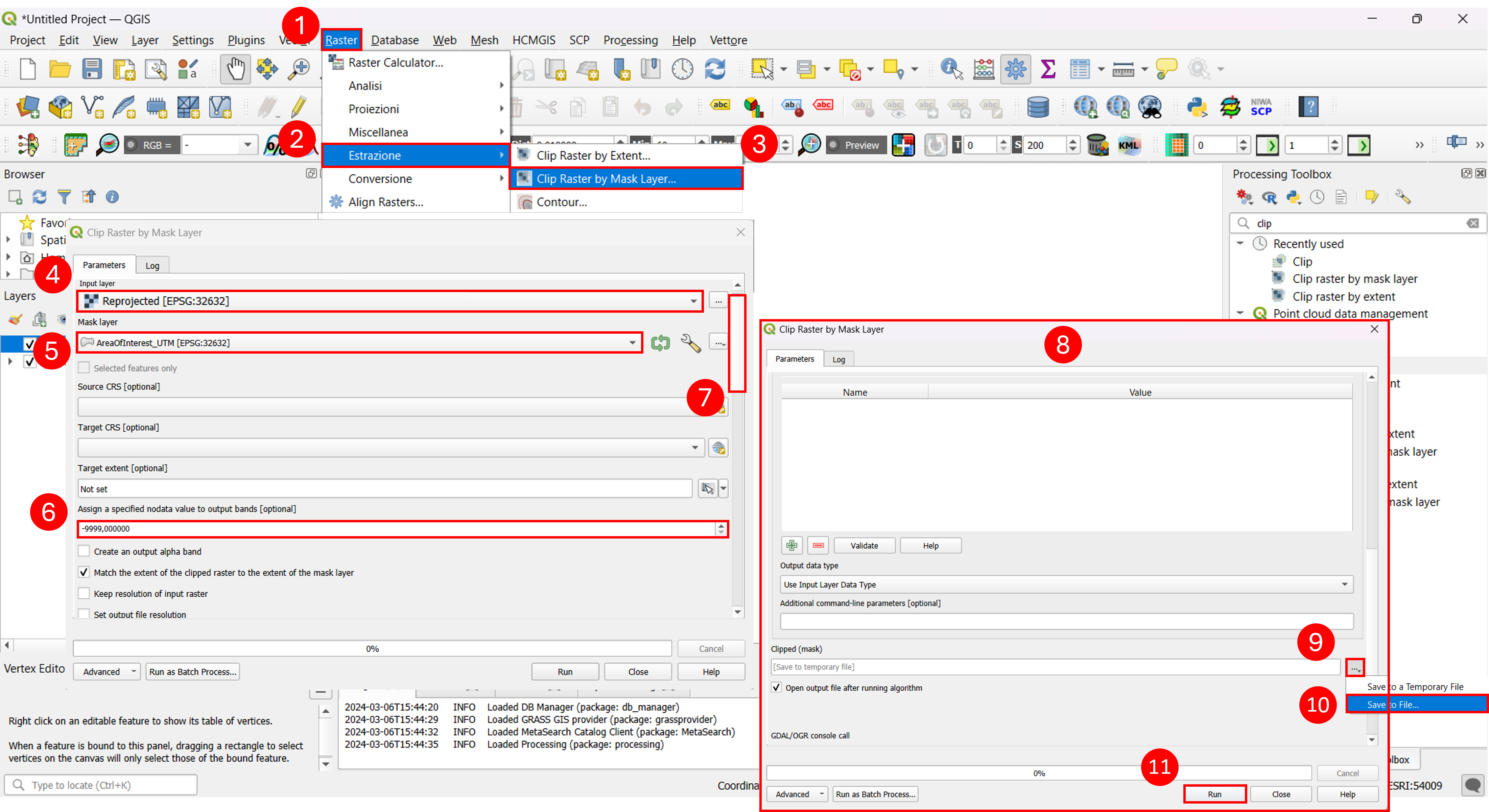
Fig. 4.1.1.2 – Clipping raster by mask layer in QGIS
Now we will visualize in a better way our clipped layer (Fig. 4.1.1.3) . Open the Layer Properties menu of the clipped layer (1), click on Symbology (2) and choose the “Singleband Pseudocolor“ Render type (3). Choose the Interpolation type as “Discrete” (4), change the Color ramp to one you like (5) and set the Label precision to “0” (6). Set the Mode field as “Continuous” (7) and click on Ok (8).
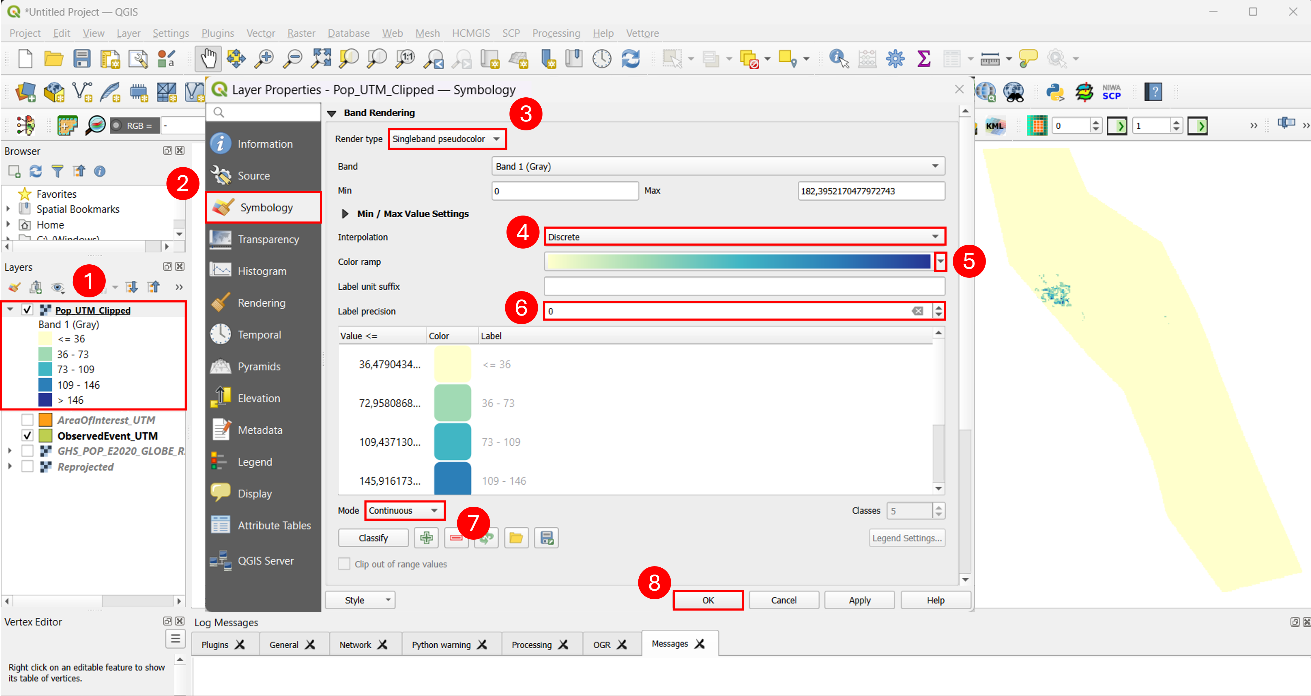
Fig. 4.1.1.3 – Visualization of GHSL-JRC population data in QGIS
If you’d like to know the population value in a specific point, you can use the Identify Features tool (Fig. 4.1.1.4) , click on it (1). Zoom-in on the area with the highest population density and click on a point where you are interested to know the population value (2). A menu called Identify Result will pop up on the right of the screen, from there you can read the population value (4).

Fig. 4.1.1.4 – identify tool in QGIS